I had five benchmark harnesses and they did not agree with each other

Every measurement project I started grew its own scripts. That is how these things go. You need one number, you write forty lines to get it, the forty lines work, and eight months later there are five separate piles of them and each pile knows a slightly different set of tricks.

The moment it became a problem was mundane. Two results disagreed by a few percent and I could not tell whether that was the machine or the code that measured the machine. Both piles were mine. Neither recorded enough about the run to settle it.

That is the failure I want to describe, because it is quiet and it does not throw an error. A harness that measures the wrong thing consistently looks exactly like a harness that measures the right thing.

What went wrong in the piles

Nothing recorded the state of the machine. A benchmark result is a number about a piece of hardware in a particular physical condition: a temperature, a clock frequency, a throttle state, whatever else was running. Four of the five piles recorded the number and threw the condition away.

A parser bug meant re-running the experiment. The scripts parsed the tool’s output inline and kept only the result. So a mistake in the parsing meant hours of measurement had to happen again, on hardware I had to physically go and use.

A failure left no trace. A run that crashed simply produced no row. Later, looking at a results directory, there is no way to tell a configuration that was never attempted from one that was attempted and died.

Adding a machine meant writing code. Each pile knew about the machines it grew up on. Getting a fifth pile onto the Raspberry Pi meant porting it.

Rebuilding it as one thing

So I rewrote all five as one framework. One configuration file names the machines, the models and the sweep. One command runs it.

The design decisions that actually earned their keep:

Every run writes a self-describing record. Hardware, kernel, compiler, backend version, model, quantization, the metrics, and the physical state of the machine while they were measured: power, temperature, clocks, throttle flags, processor utilisation. Anything the platform cannot measure is recorded as absent rather than as zero, which sounds pedantic until you try to average a column of zeroes that meant “no sensor”.

Raw output is kept. Parsing happens on the host afterwards, so a parser bug is a re-parse rather than a re-run.

Failures are records too. A crashed configuration writes a record saying it crashed.

A new machine is a config block. A hostname, an SSH key and the paths to its models. The agent that runs on the device under test uses nothing but the standard library, and nothing crosses the network inside a measurement window.

The test that mattered

A framework that produces different numbers from the scripts it replaced is worthless, however tidy it is. So the first thing I did was backfill the previous campaign’s raw measurements into the new record format and check that the analysis layer reproduced its published fits.

It did, exactly. Then I ran the whole campaign again, natively, weeks later, on the same board.

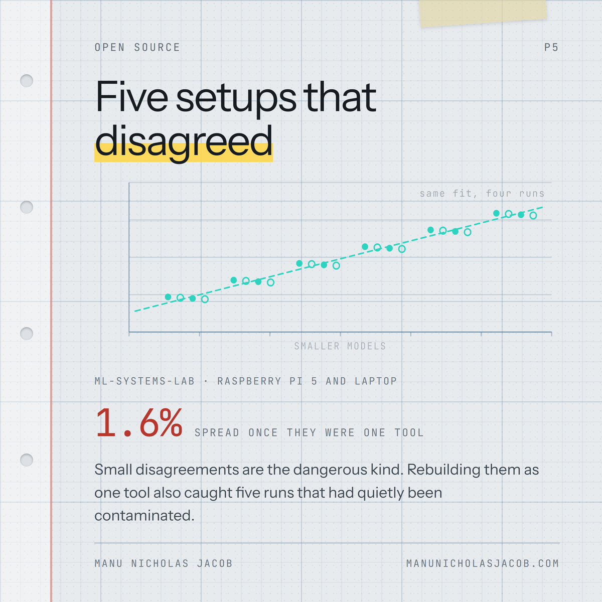
Two independent campaigns, different code, weeks apart, landing within about 1.7 percent of each other on the quantity the whole research programme rests on. The laptop half came out at 35.7 gigabytes per second both times.

That agreement is the only reason I trust either number.

The one that caught a real problem

The framework flags any run whose repetitions spread more than a threshold, and during the first Pi campaign five points in the power block tripped it. Their spread was between 30 and 103 percent against a campaign norm under 2.5 percent.

Something else had been running on the machine. Under the old scripts those five points would have gone quietly into an average and shifted a published number by a few percent, and nothing would ever have flagged them. They were deleted and re-measured on an idle board.

There is nothing clever about the flag. A standard deviation and a threshold, which is a first-year exercise. It works only because the record carries enough about the run to compute it at all, and that was the part the old scripts were missing.

Two facts that fell out for free

Once every machine speaks the same configuration file, comparisons that used to be projects become one run.

The same config shows a laptop’s graphics card losing to its own processor at one request at a time, 12.3 milliseconds against 3.0, because the cost of dispatching work to the card dominates. At sixty-four requests at once the same card wins by 29 times, 9,885 inferences a second against 338. Both numbers come out of one file, which is the point.

And eight-bit quantization is about eleven times faster than 32-bit on the Raspberry Pi’s processor while being roughly three and a half times slower on the laptop’s. Same models, same runtime. Two lines in the same report.

Using it

pip install ml-systems-lab
mlsys run configs/example-smoke.yaml
mlsys report runs/smoke-test --full

Code on GitHub, archived at 10.5281/zenodo.21867055. The committed result sets under results/ are complete datasets, records and generated report together, not summaries.

If you keep a bench of machines and a pile of scripts, the question worth asking is whether any of your results could be re-derived from what your scripts wrote down. Mine could not, for four out of five. That was the whole problem.